Probably the most revolutionary-to-me thing I’ve learned in GIS/data science/computers/programming/python/yadda yadda yadda in the past 5 years is the pandas library in python (especially so, now that ESRI has introduced the spatially enabled dataframe (and its predecessor the spatial dataframe)). Pandas is self-described as “a fast, powerful, flexible and easy to use open source data analysis and manipulation tool, built on top of the Python programming language.” It’s used extensively by data engineers and scientists for wrangling data and performing statistical analysis and is used in many machine learning/AI workflows. The stuff I can do with the help of this library still blows me away on a regular basis, even though I’ve been using it almost daily for half a decade. However, in my interaction with other professional GIS individuals over the same 5 years, when I bring the topic up, I’m more often than not met with blank stares, inquisitive looks, the comment “oh yeah, I’ve heard about that, but haven’t taken the time to learn it yet”, or sheer terrified faces of people that have attempted to learn it and been discouraged by struggling to learn it without having anyone to ask questions, and then giving up. Not having other people using this stuff makes me sad; I want all my other GIS friends to discover the joy I’ve found! There are lots of courses/blogs/webinars out on the internet that can explain pandas and all the things you can do with pandas, but I haven’t personally come across anything that does a stellar job of specifically addressing the use of pandas in the ESRI GIS world. In this post, I’d like to present to my GIS friends a small intro of what we can do with these pandas dataframes and how/why it could benefit them in their work.
Get Ready
Just like my last blog article, I’ll be using JupyterLab to do all my coding today
To begin, we’ll need to import a few libraries. The normal convention when working with pandas is to import it as “pd”. While not necessary, if you look at just about anyone’s code anywhere that uses pandas, they’ll also be importing it as “pd” so you should too so we can all be on the same sheet of music, and it’s much easier to type “pd.” all over the place in your code than it is to type “pandas.” when referencing the library. We’ll also be using the ArcGIS library so we can do all our GISing.

The Dataframe
Now that we’ve got our libraries imported, we can go get some data. Instead of working with layers/tables in a map that reference data in our database, we’ll be reading the data from our database into pandas dataframes and working with these dataframes. Just like a database table or a spreadsheet, a dataframe is structured in rows/columns, but instead of being stored in a database or a file on a disk, the dataframe lives in your computer’s RAM. The pandas library provides lots of different ways to get data into a dataframe (read_sql, read_csv, read_excel, read_json are the ones I use regularly for reading my non-GIS data). Since this is an intro to using pandas with your GIS data, I’d like to introduce you to the arcgis library’s GeoAccessor class. This class contains a lot of functionality, we’ll start with using it to read our GIS data into a dataframe.
To read data from a geodatabase feature class we can use the GeoAccessor.from_featureclass() function and provide the path to the feature class and optionally the fields we’re interested in using (if we don’t specify the fields to read, it will read all of the fields in the featureclass). There are other arguments we could provide as well to limit the data in the dataframe, but for this example we’ll read all rows into the dataframe. Note that since this is the from feature class function, it will automatically read the geometry of the row into a field named SHAPE for us, we don’t need to specify it, it will automatically get read into the dataframe for us.

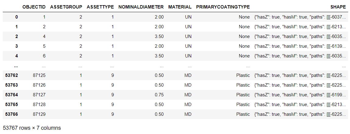
That dataframe looks similar to what we see in ArcGIS pro when we look at the attribute table when we display the same fields (other than the subtype/coded value domains not showing us their descriptions, and that first column without a header with the bold values (those bold values are the dataframe’s index, which is very important, but we can ignore it for now)):

We could also read non spatial data from a table in our database in the same manner but using the GeoAccessor’s “from_table()” function or read from a feature layer from portal or ArcGIS Online using using the GeoAccessor’s “from_layer()” function, and providing the layer’s URL.
Select By Attributes
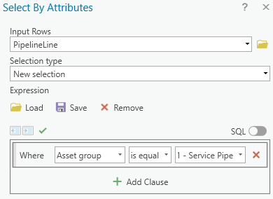
For now, let’s stick with our pipeline lines. If you wanted to select all your services in the pipeline lines feature class in ArcGIS Pro, you’d open your select by attributes window and make a where clause for Asset group is equal to 1 – Service Pipe:

To do that same selection on our dataframe we’ll use the dataframe’s .loc property

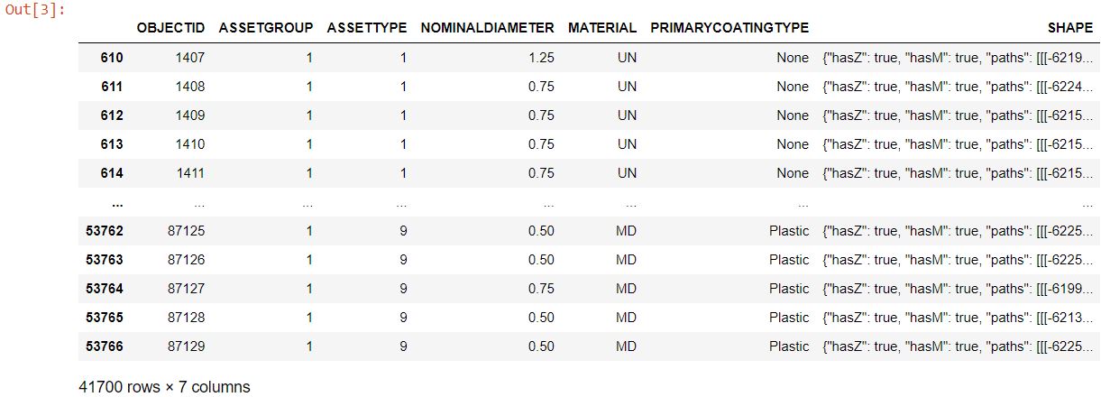
So, what happened in that cell above? it gave us the same number of rows, so clearly it worked, but if you’re coming from a background in SQL and know some python like many of us GIS professionals are, it probably looks a little strange. The first thing that seems off at first might be that the “.loc” has a square bracket after it, not a parenthesees, this is because “.loc” is a property of the dataframe, it’s not a function. Then inside the square brackets we’re giving it the dataframe again followed by more square brackets around “ASSETGROUP” ==1. Hopefully that “==1” probably makes sense, it’s just like how we test if a variable in python equals 1. lets take a closer look at that “PipelineLine_df[“ASSETGROUP”]==1″ part though. When we run PipelineLine_df[“ASSETGROUP”] we get a pandas series, which is an array of all the ASSETGROUP values in our dataframe, then the “==1” will check each of those values in the array and see if they are equal to one, and the results of that are returned as another pandas series of booleans indicating if that element in the original series is equal to one. We can take that part of the code and run it to see that it returns a series of booleans, with the same number of rows as the dataframe.


When we gave the .loc the series of booleans it spits back a copy of the dataframe but only for the rows where the bool series is True.
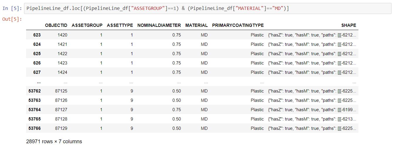
We can also use a similar approach to find only the rows in the dataframe where it is a service, and it has a material of medium density plastic
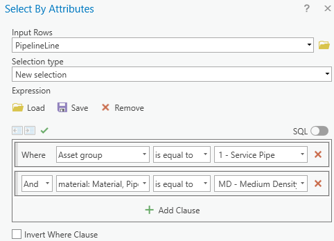

To do the same on our pandas dataframe we can just give the .loc two boolean series, one for asset group = 1 and another for the material = MD, but we’ll enclose both series in parentheses and join them together with an ampersand. (For an “or” instead of an “and” we’d use “|” instead of an ampersand)
To find rows in our dataframe where the material is either medium density or high density plastic in SQL we’d use a where clause of “MATERIAL in (‘MD’,’HD’)”. To do that in a pandas dataframe we’ll use .isin([“MD”,”HD”]) with our .loc (note that .isin() will take any list like object, so in this case we passed it a list, but we could also use a Series from another dataframe which would be analagous to a SQL subquery from another table)
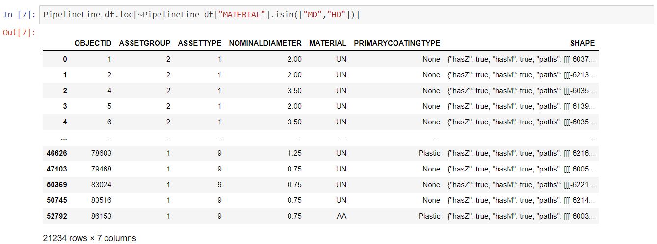
Or to get the rows where the material is not medium density or high density plastic in SQL we’d use a where clause of “MATERIAL not in (‘MD’,’HD’)”. To do that in a pandas dataframe we’ll use .isin([“MD”,”HD”]) with out .loc but we’ll flip all our Trues to Falses and vice versa with the “~” operator on the bool series
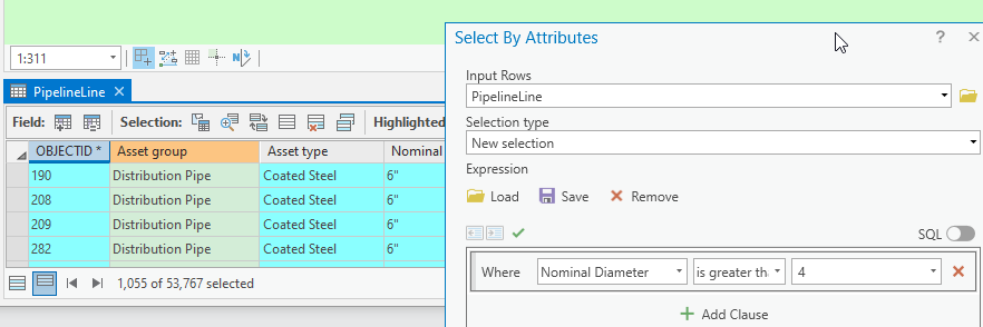
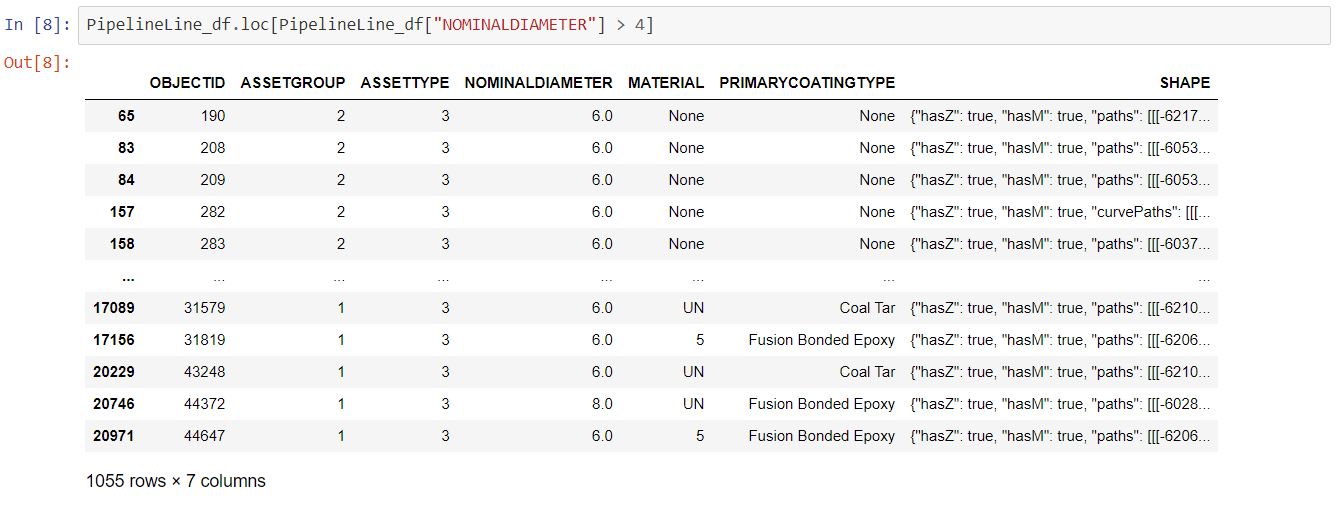
We can also do greater than, less than and that sort of query too in SQL to find lines greater than 4″ in diameter we’d use “NOMINALDIAMETER > 4”
In pandas we’ll do it like this:
Select By Location
Selecting by attributes is incredibly important, but as GIS people, we know that tabular data is not the end all be all. We like to know how things interact with one another spatially. For querying for features that intersect one another spatially in ArcGIS Pro we’d pull out our handy dandy “Select By Location” tool. In Pro I’ll draw a rectangle(ish) polygon and then select by location all my PipelineLines that intersect the polygon:

In pandas we’ll do it like this:


If you’re playing along at home (or work) and modifying this code to play with your own data, you may have noticed that that running that .spatial.select() took a lot more time to run than the select by location did in Pro. I dont want that initial selection speed discourage you! When you run that spatial select the first time, if you haven’t already created a spatial index on the dataframe (which we didn’t in this example), the arcgis python API did it for you in the background, and that took a little bit of time, but subsequent calls to the .spatial.select() function will return much much faster, because that spatial index has already been computed.
The Pandas Advantage
Since we’re working with a pandas dataframe, computing statistics on stuff is trivial (remember earlier when I said that this library is used for data engineering/analysis!). Being a small selection set we can easily look at the dataframe above and note that there is one ASSETGROUP=2 line and its MATERIAL type is ‘UN’, and there are three lines taht are ASSETGROUP=1 and two are MATERIAL ‘UN’ and one is ‘MD’. Let’s take that same selection on our lines and find out how many mains and services are of what material type. Once again after the code I’ll break it down for what’s happening.

The first thing that happened is calling the .groupby() function on the dataframe. The pandas groupby functions exactly like a group by in SQL, then after the .groupby() we specified that we wanted to take the material series and get the value counts of the groups which is essential the same as count(*) on a SQL group by. Lastly we have a .to_frame() which takes the pandas series that results from the .value_counts() and converts it to a dataframe. then the next line renames the dataframe’s columns. As expected, we get the counts we were expecting, two asset group 1 material UN, one asset group 1 material MD and one asset group 2 material UN. A keen eye will notice that when we display the dataframe that the header of the displayed dataframe has two different levels, and the first two columns are bolded. The first two columns are a multiindex. Fantastic things can happen with multiindexs but that’s out of scope for this blog post, lets just focus on the basics :).
The last thing I’d like to introduce today is replacement of values in a dataframe. since the ASSETGROUP in the database is the subtype and is stored as an integer but has a description, and the material field is text that is controlled by a coded value domain, it might be helpful to see what the descriptions are for these fields in our dataframe.

Look at that, we used the dictionaries to replace the values in the series’ with human readable text.
This is only the beginning of what is possible
Although this blog post is coming to a close, I’d like to clairify that this is only the tip of the iceburg of what you can do with pandas/GIS/spatial dataframes. I’ve been able to build data pipelines that maintain data in a GIS using pandas, create tools that do full enterprise GIS data migrations in minutes, use it to find descrepancies in existing data, and produce neat feature reports just to name a few. Once the pandas bug gets ya, you’ll see the world of data in a whole new light. If you were new to pandas when you started reading, I hope this post helped you learn something new and inspired you to give some of this stuff a shot. Until next time, Happy coding!

What do you think?