Jupyter Notebook is an increasingly popular open-source web application used by all sorts of people for all sorts of purposes. It is an easy way to work with data programmatically, repeat the work, and share it. Many data scientists use this tool, and because GIS data is just data with a spatial component, you can use it too. In fact, Esri now ships Jupyter Notebook with its software.

This article walks through using GIS data in Jupyter Notebook for the first time. We will download a sample geodatabase, download some code, do a little housekeeping, and run the code. The goal is not to create an efficient workflow, but to understand how to move the information between formats with Jupyter Notebook. We will not, for instance, use the function FeatureClassToNumPyArray in ArcPy’s Data Access module to get DataFrame objects in one shot. Nor will we touch on Spatial DataFrame objects here.

Before We Begin

There are a couple prerequisites for the instructions in this article to keep things simple. First, you are working on a Windows 10 machine. Second, your machine has an updated ArcGIS Pro install.

Download the Sample Data

Our sample data will come from the U.S. Fish and Wildlife Service. Go here, scroll down, and click download by state. Click on the state of your choice, the geodatabase option, and save.

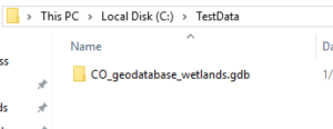
I chose Colorado and created the folder C:\TestData and unzipped the geodatabase there.

Download the Jupyter Notebook File

Go to the SSP Innovations GitHub site here. Click on raw and press ctrl + s to save it as an IPYNB file locally.

Install PySAL Using Python Package Manager

We can take advantage of the Python Package Manager that come with ArcGIS Pro to easily install the PySAL package our code requires. Boot up Pro and head to Settings.

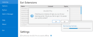
While in Settings, go to Licensing and check the box to authorize ArcGIS Pro to work offline. This will allow the code to import ArcPy without ArcGIS Pro being open.

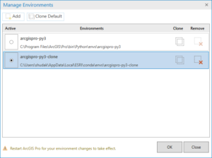
Now we will clone the default python environment so we can install some packages. Still in Settings, go to Python and click Manage Environments. Click Clone Default, type in a name if you want or keep the default and hit Clone.

It will take a bit to install the clone environment. Select the new item in the list and hit OK.

Restart ArcGIS Pro and go back to Python in Settings. Search “pysal” and click Install. In the dialogue that comes up check the box to agree and click Install. After its finished you can close ArcGIS Pro.

In ArcGIS Pro 2.3 PySAL is the only package you will need to install. At the time of writing release 1.14.4.0 is available but 2.0.0 was recently released and should be available soon.

Run Jupyter Notebook

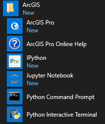
To start the Jupyter Notebook go to the ArcGIS start menu folder and open Python Command Prompt (not Jupyter Notebook).

Type “jupyter notebook” and hit return. After a moment you should see the Jupyter Notebook Dashboard in your browser. By launching this way, the PySAL package we just installed will be accessible.

Click upload in the top right side of the Dashboard and choose the IPYNB notebook file you downloaded previously.

You will see the file in the Dashboard. Click the new upload button next to it.

Now that the file is uploaded, click on it and it will open in the Notebook Editor. The code is broken up into different cells. The cells can be run separately or all at once. If you are interested in learning about the user interface you can find documentation here. Next, we will describe each section and then run the code.

Import Modules and Packages

The first cell has the import statements to make use of functions in the various modules listed.

Specify Folders

The C:\TempAnalysis folder is created, used, and removed as the code runs. The folder at C:\TestData is the folder created earlier when the data was downloaded.

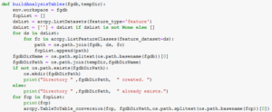
Build Temporary Workspace

Check for the existence of the temporary folder mentioned above and if it doesn’t exist create it. A message stating the true condition prints.

Build Analysis Database List

Create a list of file geodatabases in the data folder using the ArcPy Function ListWorkspaces.

Build Analysis Tables

Create a list of feature classes by searching the top level of the geodatabase and all datasets. Note that this ignores object classes in the database. After the list is created, an ArcPy function is called to write a DBF file into the temporary folder from each feature class found in the geodatabase.

Build DBF Location List

Build a list of the locations of the DBF files.

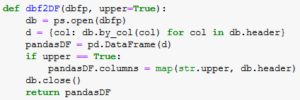
DBF to DataFrame

Read in the DBF file, convert it to a dictionary, convert the dictionary to a Pandas DataFrame, and make the columns uppercase in the returned DataFrame.

DBF Iterate

Iterate through the list of DBF file locations, run the function ‘dbf2DF’, and display the returned DataFrame object using PySAL for each DBF file.

FGDB Iterate

Iterate through the list of geodatabases and run the function ‘dbfIterate’ with the output of the function ‘buildDBFPList’ as its parameter for each database.

Cleanup Temporary Workspace

Check for the existence of the temporary folder. If it exists, delete the folder and all contains.

Execute the Functions

Results Display

Each DataFrame object created from the feature classes in the geodatabase are displayed in the notebook.

Run the Notebook

While in the Notebook Dashboard click Cell and Run All. Errors will report in the appropriate cell if any occur. An asterisk will display next to the cell while it is running. Information will print out at the bottom and the data will display below that. Depending on the size of the wetlands data downloaded it may take a minute or so.

The interesting feat accomplished in this notebook is the conversion of data from one form to another. Moving the data out of narrow file formats for data integration or analysis can be useful and Jupyter Notebook is a convenient way to run and share these processes.